import emat
emat.versions()

emat 0.5.1, plotly 4.14.3

Feature Scoring

Feature scoring is a methodology for identifying what model inputs (in machine learning terminology, “features”) have the greatest relationship to the outputs.

The relationship is not necessarily linear, but rather can be any arbitrary linear or non-linear relationship. For example, consider the function:

import numpy

def demo(A=0,B=0,C=0,**unused):
    """
    Y = A/2 + sin(6πB) + ε
    """
    return {'Y':A/2 + numpy.sin(6 * numpy.pi * B) + 0.1 * numpy.random.random()}

We can readily tell from the functional form that the B term is the most significant when all parameter vary in the unit interval, as the amplitude of the sine wave attached to B is 1 (although the relationship is clearly non-linear) while the maximum change in the linear component attached to A is only one half, and the output is totally unresponsive to C.

To demonstrate the feature scoring, we can define a scope to explore this demo model:

demo_scope = emat.Scope(scope_file='', scope_def="""---
scope:
    name: demo
inputs:
    A:
        ptype: exogenous uncertainty
        dtype: float
        min: 0
        max: 1
    B:
        ptype: exogenous uncertainty
        dtype: float
        min: 0
        max: 1
    C:
        ptype: exogenous uncertainty
        dtype: float
        min: 0
        max: 1
outputs:
    Y:
        kind: info
""")

And then we will design and run some experiments to generate data used for feature scoring.

from emat import PythonCoreModel
demo_model = PythonCoreModel(demo, scope=demo_scope)
experiments = demo_model.design_experiments(n_samples=5000)
experiment_results = demo_model.run_experiments(experiments)

The feature_scores() method from the emat.analysis subpackage allows for feature scoring based on the implementation found in the EMA Workbench.

from emat.analysis import feature_scores
fs = feature_scores(demo_scope, experiment_results)
fs

	A	B	C
Y	0.136464	0.784930	0.078605

Note that the feature_scores() depend on the scope (to identify what are input features and what are outputs) and the experiment_results, but not on the model itself.

We can plot each of these input parameters using the display_experiments method, which can help visualize the underlying data and exactly how B is the most important feature for this example.

from emat.analysis import display_experiments
fig = display_experiments(demo_scope, experiment_results, render=False, return_figures=True)['Y']
fig.update_layout(
    xaxis_title_text =f"A (Feature Score = {fs.data.loc['Y','A']:.3f})",
    xaxis2_title_text=f"B (Feature Score = {fs.data.loc['Y','B']:.3f})",
    xaxis3_title_text=f"C (Feature Score = {fs.data.loc['Y','C']:.3f})",
)
from emat.util.rendering import render_plotly
render_plotly(fig, '.png')

One important thing to consider is that changing the range of the input parameters in the scope can significantly impact the feature scores, even if the underlying model itself is not changed. For example, consider what happens to the features scores when we expand the range of the uncertainties:

demo_model.scope = emat.Scope(scope_file='', scope_def="""---
scope:
    name: demo
inputs:
    A:
        ptype: exogenous uncertainty
        dtype: float
        min: 0
        max: 5
    B:
        ptype: exogenous uncertainty
        dtype: float
        min: 0
        max: 5
    C:
        ptype: exogenous uncertainty
        dtype: float
        min: 0
        max: 5
outputs:
    Y:
        kind: info
""")

wider_experiments = demo_model.design_experiments(n_samples=5000)
wider_results = demo_model.run_experiments(wider_experiments)

from emat.analysis import feature_scores
wider_fs = feature_scores(demo_model.scope, wider_results)
wider_fs

	A	B	C
Y	0.772328	0.158978	0.068695

fig = display_experiments(demo_model.scope, wider_results, render=False, return_figures=True)['Y']
fig.update_layout(
    xaxis_title_text =f"A (Feature Score = {wider_fs.data.loc['Y','A']:.3f})",
    xaxis2_title_text=f"B (Feature Score = {wider_fs.data.loc['Y','B']:.3f})",
    xaxis3_title_text=f"C (Feature Score = {wider_fs.data.loc['Y','C']:.3f})",
)
render_plotly(fig, '.png')

The pattern has shifted, with the sine wave in B looking much more like the random noise, while the linear trend in A is now much more important in predicting the output, and the feature scores also shift to reflect this change.

Road Test Feature Scores

We can apply the feature scoring methodology to the Road Test example in a similar fashion. To demonstrate scoring, we’ll first load and run a sample set of experients.

from emat.model.core_python import Road_Capacity_Investment
road_scope = emat.Scope(emat.package_file('model','tests','road_test.yaml'))
road_test = PythonCoreModel(Road_Capacity_Investment, scope=road_scope)
road_test_design = road_test.design_experiments(sampler='lhs')
road_test_results = road_test.run_experiments(design=road_test_design)

With the experimental results in hand, we can use the same feature_scores() function to compute the scores.

feature_scores(road_scope, road_test_results)

	alpha	beta	input_flow	value_of_time	unit_cost_expansion	interest_rate	yield_curve	expand_capacity	amortization_period	debt_type	interest_rate_lock
no_build_travel_time	0.075293	0.068182	0.538393	0.046090	0.043536	0.045446	0.042912	0.041798	0.039350	0.030986	0.028014
build_travel_time	0.046962	0.047576	0.294707	0.048980	0.051786	0.061001	0.053346	0.274514	0.047741	0.038547	0.034840
time_savings	0.082390	0.089531	0.437443	0.046821	0.051698	0.050382	0.046855	0.086983	0.048425	0.030447	0.029026
value_of_time_savings	0.080125	0.064977	0.296455	0.196913	0.043270	0.051546	0.051619	0.086728	0.045814	0.043878	0.038676
net_benefits	0.073350	0.048033	0.274585	0.116004	0.048006	0.043684	0.058289	0.189976	0.065641	0.044471	0.037961
cost_of_capacity_expansion	0.037718	0.034734	0.048601	0.042841	0.084262	0.039434	0.044483	0.494295	0.103566	0.040153	0.029912
present_cost_expansion	0.038055	0.025013	0.029004	0.029836	0.086967	0.039247	0.035163	0.649856	0.025137	0.021536	0.020184

By default, the feature_scores() function returns a stylized DataFrame, but we can also use the return_type argument to get a plain ‘dataframe’ or a rendered svg ‘figure’.

feature_scores(road_scope, road_test_results, return_type='dataframe')

	alpha	beta	input_flow	value_of_time	unit_cost_expansion	interest_rate	yield_curve	expand_capacity	amortization_period	debt_type	interest_rate_lock
no_build_travel_time	0.076455	0.067577	0.547147	0.038260	0.048396	0.042603	0.043010	0.038458	0.041105	0.032364	0.024624
build_travel_time	0.047886	0.051504	0.279975	0.060721	0.055445	0.053489	0.044081	0.300634	0.049298	0.027803	0.029163
time_savings	0.108482	0.069877	0.446738	0.040805	0.052594	0.046389	0.044383	0.085607	0.039477	0.036638	0.029010
value_of_time_savings	0.080945	0.070036	0.318382	0.156613	0.043204	0.047959	0.067452	0.089235	0.059085	0.037841	0.029249
net_benefits	0.066060	0.056216	0.271768	0.121979	0.054652	0.048983	0.047650	0.177654	0.077722	0.046306	0.031012
cost_of_capacity_expansion	0.034423	0.038636	0.043843	0.040750	0.080650	0.047269	0.045473	0.492494	0.106107	0.045416	0.024940
present_cost_expansion	0.031402	0.029665	0.026294	0.030246	0.081330	0.036982	0.024279	0.664286	0.029862	0.025960	0.019693

feature_scores(road_scope, road_test_results, return_type='figure')

The colors on the returned DataFrame highlight the most important input features for each performance measure (i.e., in each row). The yellow highlighted cell indicates the most important input feature for each output feature, and the other cells are colored from yellow through green to blue, showing high-to-low importance. These colors are from matplotlib’s default “viridis” colormap. A different colormap can be used by giving a named colormap in the cmap argument.

feature_scores(road_scope, road_test_results, cmap='copper')

	alpha	beta	input_flow	value_of_time	unit_cost_expansion	interest_rate	yield_curve	expand_capacity	amortization_period	debt_type	interest_rate_lock
no_build_travel_time	0.067907	0.068892	0.545381	0.039791	0.048858	0.044914	0.038852	0.043290	0.039698	0.032160	0.030257
build_travel_time	0.040019	0.047880	0.286568	0.039084	0.048906	0.049377	0.055488	0.316152	0.042957	0.044400	0.029169
time_savings	0.083301	0.079282	0.433071	0.047197	0.049545	0.049384	0.053214	0.093971	0.043185	0.033031	0.034819
value_of_time_savings	0.084197	0.066246	0.315413	0.189313	0.051799	0.043885	0.054402	0.067124	0.054650	0.036482	0.036488
net_benefits	0.065213	0.062103	0.251974	0.117954	0.054434	0.045045	0.067021	0.191905	0.075528	0.040360	0.028463
cost_of_capacity_expansion	0.040910	0.037305	0.049215	0.040266	0.081726	0.046242	0.045754	0.489732	0.095459	0.044652	0.028739
present_cost_expansion	0.027351	0.017587	0.025910	0.028115	0.085811	0.032409	0.026658	0.674268	0.032287	0.027821	0.021783

You may also notice small changes in the numbers given in the two tables above. This occurs because the underlying algorithm for scoring uses a random trees algorithm. If you need to have stable (replicable) results, you can provide an integer in the random_state argument.

feature_scores(road_scope, road_test_results, random_state=1, cmap='bone')

	alpha	beta	input_flow	value_of_time	unit_cost_expansion	interest_rate	yield_curve	expand_capacity	amortization_period	debt_type	interest_rate_lock
no_build_travel_time	0.069742	0.067682	0.557708	0.038260	0.037500	0.043854	0.039635	0.045330	0.046019	0.029962	0.024308
build_travel_time	0.038978	0.052516	0.294415	0.036316	0.042900	0.048776	0.049931	0.331223	0.040332	0.030027	0.034586
time_savings	0.084854	0.084775	0.427335	0.056313	0.045476	0.050672	0.041260	0.090572	0.047126	0.040557	0.031062
value_of_time_savings	0.076504	0.055238	0.334227	0.177406	0.045623	0.038967	0.071869	0.075423	0.046744	0.043492	0.034506
net_benefits	0.068594	0.050820	0.270457	0.113781	0.049488	0.051259	0.069530	0.181702	0.077212	0.036118	0.031038
cost_of_capacity_expansion	0.038307	0.036459	0.044803	0.049044	0.076379	0.039507	0.043260	0.489785	0.119787	0.038756	0.023914
present_cost_expansion	0.032561	0.032959	0.038989	0.040957	0.107123	0.041828	0.040684	0.588281	0.025878	0.030009	0.020731

Then if we call the function again with the same random_state, we get the same numerical result.

feature_scores(road_scope, road_test_results, random_state=1, cmap='YlOrRd')

	alpha	beta	input_flow	value_of_time	unit_cost_expansion	interest_rate	yield_curve	expand_capacity	amortization_period	debt_type	interest_rate_lock
no_build_travel_time	0.069742	0.067682	0.557708	0.038260	0.037500	0.043854	0.039635	0.045330	0.046019	0.029962	0.024308
build_travel_time	0.038978	0.052516	0.294415	0.036316	0.042900	0.048776	0.049931	0.331223	0.040332	0.030027	0.034586
time_savings	0.084854	0.084775	0.427335	0.056313	0.045476	0.050672	0.041260	0.090572	0.047126	0.040557	0.031062
value_of_time_savings	0.076504	0.055238	0.334227	0.177406	0.045623	0.038967	0.071869	0.075423	0.046744	0.043492	0.034506
net_benefits	0.068594	0.050820	0.270457	0.113781	0.049488	0.051259	0.069530	0.181702	0.077212	0.036118	0.031038
cost_of_capacity_expansion	0.038307	0.036459	0.044803	0.049044	0.076379	0.039507	0.043260	0.489785	0.119787	0.038756	0.023914
present_cost_expansion	0.032561	0.032959	0.038989	0.040957	0.107123	0.041828	0.040684	0.588281	0.025878	0.030009	0.020731

Interpreting Feature Scores

The correct interpretation of feature scores is obviously important. As noted above, the feature scores can reveal both linear and non-linear relationships. But the scores themselves give no information about which is which.

In addition, while the default feature scoring algorithm generates scores that total to 1.0, it does not necessarily map to dividing up the explained variance. Factors that have little to no effect on the output still are given non-zero feature score values. You can see an example of this in the “demo” function above; that simple example literally ignores the “C” input, but it has a non-zero score assigned. If there are a large number of superfluous inputs, they will appear to reduce the scores attached to the meaningful inputs.

It is also important to remember that these scores do not fully reflect any asymmetric relationships in the data. A feature may be very important for some portion of the range of a performance measure, and less important in other parts of the range. For example, in the Road Test model, the “expand_capacity” lever has a highly asymmetric impact on the “net_benefits” measure: it is very important in determining negative values (when congestion isn’t going to be bad due to low “input_flow” volumes, the net loss is limited by how much we spend), but not so important for positive values (nearly any amount of expansion has a big payoff if congestion is going to be bad due to high “input_flow” volume). If we plot this three-way relationship specifically, we can observe it on one figure:

from matplotlib import pyplot as plt
fig, ax = plt.subplots()
ax = road_test_results.plot.scatter(
    c='net_benefits',
    y='expand_capacity',
    x='input_flow',
    cmap='coolwarm',
    ax=ax,
)

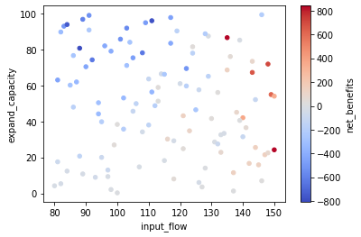
Looking at the figure above, we can see the darker red clustered to the right, and the darker blue clustered in the top left. However, if we are not aware of this particular three-way relationship a priori, it may be difficult to discover it by looking through various combinations of three-way relationships. To uncover this kind of relationship, threshold scoring may be useful.

Threshold Scoring

Threshold scoring provides a set of feature scores that don’t relate to the overall magnitude of a performance measure, but rather whether that performance measure is above or below some threshold level. The threshold_feature_scores() function computes such scores for a variety of different thresholds, to develop a picture of the relationship across the range of outputs.

from emat.analysis.feature_scoring import threshold_feature_scores

threshold_feature_scores(road_scope, 'net_benefits', road_test_results)

	-596.2998419053935	-532.2177460113968	-468.1356501174002	-404.0535542234036	-339.9714583294069	-275.88936243541025	-211.80726654141364	-147.72517064741703	-83.64307475342036	-19.5609788594237	44.52111703457297	108.60321292856952	172.68530882256618	236.76740471656285	300.8495006105594	364.93159650455607	429.01369239855273	493.0957882925494	557.1778841865461	621.2599800805428
alpha	0.075148	0.050279	0.059898	0.103448	0.117437	0.077087	0.059059	0.065693	0.045667	0.072984	0.079683	0.078461	0.063940	0.071503	0.067585	0.101356	0.084803	0.076406	0.091555	0.075858
beta	0.062863	0.065949	0.071284	0.070418	0.041685	0.053184	0.055833	0.057309	0.060744	0.055626	0.061131	0.069423	0.087561	0.087615	0.093054	0.061921	0.076819	0.111758	0.075494	0.077963
input_flow	0.099042	0.117610	0.121540	0.133525	0.157956	0.202672	0.194030	0.178355	0.203482	0.291356	0.328865	0.281785	0.262936	0.256167	0.221948	0.221820	0.186323	0.224079	0.236539	0.202316
value_of_time	0.092756	0.090173	0.070189	0.052254	0.061863	0.079276	0.053757	0.073133	0.104445	0.137612	0.088578	0.097355	0.138259	0.137003	0.136594	0.152264	0.184779	0.188427	0.180954	0.166136
unit_cost_expansion	0.101838	0.079997	0.072786	0.052329	0.058754	0.076293	0.068773	0.052392	0.055921	0.064583	0.068868	0.070714	0.067171	0.050264	0.047013	0.045760	0.062143	0.058584	0.053345	0.080208
interest_rate	0.060629	0.055555	0.064587	0.057517	0.058705	0.055403	0.060793	0.053051	0.072146	0.063817	0.075683	0.079550	0.073380	0.059745	0.071573	0.058264	0.047997	0.070229	0.071760	0.061203
yield_curve	0.056337	0.085194	0.083580	0.061164	0.054890	0.046631	0.060609	0.054925	0.063682	0.062777	0.074276	0.076540	0.104534	0.100175	0.105485	0.131876	0.132665	0.071773	0.091659	0.099439
expand_capacity	0.125463	0.210470	0.260424	0.307043	0.240281	0.248223	0.294557	0.318593	0.237247	0.105743	0.064666	0.068426	0.045452	0.052989	0.052125	0.046287	0.084356	0.057788	0.057288	0.094136
amortization_period	0.209180	0.172479	0.103268	0.073847	0.103093	0.083261	0.070993	0.071950	0.060059	0.063213	0.056224	0.080024	0.060268	0.088706	0.090940	0.104742	0.059355	0.068531	0.058589	0.071917
debt_type	0.076596	0.039295	0.063979	0.061042	0.072186	0.049546	0.046141	0.046417	0.059387	0.047572	0.055698	0.055564	0.049843	0.047698	0.065033	0.034613	0.039652	0.035859	0.042966	0.041564
interest_rate_lock	0.040149	0.032998	0.028465	0.027412	0.033151	0.028425	0.035455	0.028181	0.037222	0.034716	0.046327	0.042159	0.046656	0.048133	0.048650	0.041097	0.041108	0.036564	0.039851	0.029260

This table of data may be overwhelming even for an analyst to interpret, but the threshold_feature_scores() function also offers a violin or ridgeline style figure that displays similar information in a more digestible format.

threshold_feature_scores(road_scope, 'net_benefits', road_test_results, return_type='figure.png')

threshold_feature_scores(road_scope, 'net_benefits', road_test_results, return_type='ridge figure.svg')

In these figures, we can see that “expand_capacity” is important for negative outcomes, but for positive outcomes we should focus more on “input_flow”, and to a lesser but still meaningful extent also “value_of_time”.

Feature Scoring API

emat.analysis.feature_scoring.feature_scores(scope, design, return_type='styled', db=None, random_state=None, cmap='viridis', measures=None, shortnames=None)

Calculate feature scores based on a design of experiments.

Parameters:

• scope (emat.Scope) – The scope that defines this analysis.
• design (str or pandas.DataFrame) – The name of the design of experiments to use for feature scoring, or a single pandas.DataFrame containing the experimental design and results.
• return_type ({‘styled’, ‘figure’, ‘dataframe’}) – The format to return, either a heatmap figure as an SVG render in and xmle.Elem, or a plain pandas.DataFrame, or a styled dataframe.
• db (emat.Database) – If design is given as a string, extract the experiments from this database.
• random_state (int or numpy.RandomState, optional) – Random state to use.
• cmap (string or colormap, default ‘viridis’) – matplotlib colormap to use for rendering.
• measures (Collection, optional) – The performance measures on which feature scores are to be generated. By default, all measures are included.
• shortnames (Scope or callable) – If given, use this function to convert the measure names into more readable shortname values from the scope, or by using a function that maps measures names to something else.

Returns:

Returns a rendered SVG as xml, or a DataFrame, depending on the return_type argument.

Return type:

xmle.Elem or pandas.DataFrame

This function internally uses feature_scoring from the EMA Workbench, which in turn scores features using the “extra trees” regression approach.

emat.analysis.feature_scoring.threshold_feature_scores(scope, measure_name, design, return_type='styled', *, db=None, random_state=None, cmap='viridis', z_min=0, z_max=1, min_tail=5, max_breaks=20, break_spacing='linear')

Compute and display threshold feature scores for a performance measure.

This function is useful to detect and understand non-linear relationships between performance measures and various input parameters.

Parameters:

• scope (emat.Scope) – The scope that defines this analysis.
• measure_name (str) – The name of an individual performance measure to analyze.
• design (str or pandas.DataFrame) – The name of the design of experiments to use for feature scoring, or a single pandas.DataFrame containing the experimental design and results.
• return_type (str) – The format to return: - ‘dataframe’ gives a plain pandas.DataFrame, - ‘styled’ gives a colorized pandas.DataFrame, - ‘figure’ gives a plotly violin plot, - ‘ridge figure’ gives a plotly ridgeline figure. Either plotly result can optionally have “.svg” or “.png” added to render a static image in those formats.
• db (emat.Database) – If design is given as a string, extract the experiments from this database.
• random_state (int or numpy.RandomState, optional) – Random state to use.
• cmap (string or colormap, default ‘viridis’) – matplotlib colormap to use for rendering. Ignored if return_type is ‘dataframe’.
• z_min (float, optional) – Trim the bottom and top of the colormap range, respectively. Defaults to (0,1) which will make the most relevant overall feature colored at the top of the colorscale and the least relevant feature at the bottom.
• z_max (float, optional) – Trim the bottom and top of the colormap range, respectively. Defaults to (0,1) which will make the most relevant overall feature colored at the top of the colorscale and the least relevant feature at the bottom.
• min_tail (int, default 5) – The minimum number of observations on each side of any threshold point. If this value is too small, the endpoint feature scoring results are highly unstable, but if it is too large then important nonlinearities near the extreme points may not be detected. This is also used as the minimum average number of observations between threshold points.
• max_breaks (int, default 20) – The maximum number of distinct threshold points to use. Setting this value higher improves resolution but also requires more computational time.
• break_spacing ({‘linear’, ‘percentile’}) – How to distribute threshold breakpoints to test within the min-max range.

Returns:

plotly.Figure or DataFrame or styled DataFrame