import emat
emat.versions()

emat 0.5.2, plotly 4.14.3

Experimental Designs

A fundamental part of TMIP-EMAT is the development of a “design of experiments” to use in conjunction with a model. The experimental design lays out a list of model experiments to be conducted, and can be constructed in a number of different ways: it can be a systematic design, a random design, or something in between.

Developing an experimental design using TMIP-EMAT requires that an exploratory scope is defined, to identify the model inputs and their potential values. To illustrate designs, we’ll work with the scope from the road test model.

import emat.examples
scope, db, model = emat.examples.road_test()

Univariate Sensitivity Tests

One of the simplest experimental designs, and one used often in practice for transportation models, is a series of univariate sensitivity tests. In this design, a set of baseline or default model inputs is used as a starting point, and then input parameters are changed one at a time to non-default values. Univariate sensitivity tests are excellent tools for debugging and quality checking the model code, as they allow modelers to confirm that each modeled input is (or is intentionally not) triggering some change in the model outputs.

TMIP-EMAT provides the design_sensitivity_tests function to automatically generate a design of univariate sensitivity tests, given an exploratory scope. This tool will systematically generate experiments where all of the inputs but one are set to their default values, and the holdout input is then set to alternative values. For numerical inputs, the alternative values are the minimum or maximum value (one experiment for each, if they are different from the default). For categorical and boolean inputs, one experiment is created for each possible input value.

from emat.experiment.experimental_design import design_sensitivity_tests
ust = design_sensitivity_tests(scope, design_name='univariate_tests')
ust

	free_flow_time	initial_capacity	alpha	beta	input_flow	value_of_time	unit_cost_expansion	interest_rate	yield_curve	expand_capacity	amortization_period	debt_type	interest_rate_lock
0	60	100	0.15	4.0	100	0.075	100	0.030	0.0100	10.0	30	GO Bond	False
1	60	100	0.10	4.0	100	0.075	100	0.030	0.0100	10.0	30	GO Bond	False
2	60	100	0.20	4.0	100	0.075	100	0.030	0.0100	10.0	30	GO Bond	False
3	60	100	0.15	3.5	100	0.075	100	0.030	0.0100	10.0	30	GO Bond	False
4	60	100	0.15	5.5	100	0.075	100	0.030	0.0100	10.0	30	GO Bond	False
5	60	100	0.15	4.0	80	0.075	100	0.030	0.0100	10.0	30	GO Bond	False
6	60	100	0.15	4.0	150	0.075	100	0.030	0.0100	10.0	30	GO Bond	False
7	60	100	0.15	4.0	100	0.001	100	0.030	0.0100	10.0	30	GO Bond	False
8	60	100	0.15	4.0	100	0.250	100	0.030	0.0100	10.0	30	GO Bond	False
9	60	100	0.15	4.0	100	0.075	95	0.030	0.0100	10.0	30	GO Bond	False
10	60	100	0.15	4.0	100	0.075	145	0.030	0.0100	10.0	30	GO Bond	False
11	60	100	0.15	4.0	100	0.075	100	0.025	0.0100	10.0	30	GO Bond	False
12	60	100	0.15	4.0	100	0.075	100	0.040	0.0100	10.0	30	GO Bond	False
13	60	100	0.15	4.0	100	0.075	100	0.030	-0.0025	10.0	30	GO Bond	False
14	60	100	0.15	4.0	100	0.075	100	0.030	0.0200	10.0	30	GO Bond	False
15	60	100	0.15	4.0	100	0.075	100	0.030	0.0100	0.0	30	GO Bond	False
16	60	100	0.15	4.0	100	0.075	100	0.030	0.0100	100.0	30	GO Bond	False
17	60	100	0.15	4.0	100	0.075	100	0.030	0.0100	10.0	15	GO Bond	False
18	60	100	0.15	4.0	100	0.075	100	0.030	0.0100	10.0	50	GO Bond	False
19	60	100	0.15	4.0	100	0.075	100	0.030	0.0100	10.0	30	Rev Bond	False
20	60	100	0.15	4.0	100	0.075	100	0.030	0.0100	10.0	30	Paygo	False
21	60	100	0.15	4.0	100	0.075	100	0.030	0.0100	10.0	30	GO Bond	True

The output of this function is an emat.ExperimentalDesign, which is a subclass of a typical pandas DataFrame. The emat.ExperimentalDesign subclass attaches some useful metadata to the actual contents of the design, namely:

• sampler_name, which for univariate sensitivity test is 'uni',
• design_name, a descriptive name for storing and retrieving experiments and results in a database, and
• scope, which contains a reference to the scope used to define this design.

ust.scope is scope

True

ust.sampler_name

'uni'

ust.design_name

'univariate_tests'

Efficient Designs

The univariate tests, while useful for model debugging and testing, are not the best choice for exploratory modeling, where we want to consider changing many input factors at once. To support multivariate exploratation, TMIP-EMAT includes a design_experiments function that offers several different multivariate samplers.

from emat.experiment.experimental_design import design_experiments

The default multivariate sampler is a basic Latin Hypercube sampler. Meta-models for deterministic simulation experiments, such as a TDM, are best supported by a “space filling” design of experiments, such as Latin Hypercube draws (Sacks, Welch, Mitchell, & Wynn, 1989).

A Latin Hypercube sample for one dimension is constructed by subdividing the distribution of each input factor into N equally probable ranges, and drawing one random sample within each range. For example, if an input factor is assumed to be uniformly distributed between 0.1 and 0.2, that distribution can be divided into four regions (0.1-0.125, 0.125-0.15, 0.15-0.175, and 0.175-0.2), and one random draw can be made in each region. In the example below, we illustrate exactly this, for the “alpha” parameter in the demo scope.

n=4
design = design_experiments(scope, n_samples=n, random_seed=0)
ax = design.plot.scatter(x='alpha', y='initial_capacity', grid=True, figsize=(6,1))
xlim = design.scope['alpha'].range
ax.set_xlim(xlim)
ax.set_xticks(np.linspace(*xlim, n+1))
ax.set_ylabel('')
ax.set_yticks([]);

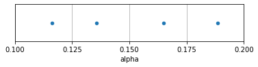
This ensures better coverage of the entire input range than making four random draws from the full space, which could easily result in a cluster of observations in one part of the space and large void elsewhere.

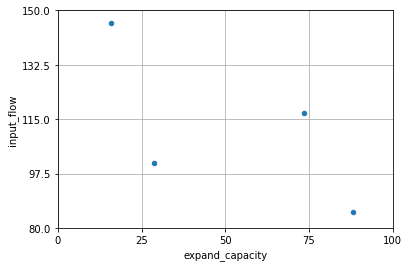
Generating a multi-dimensional Latin Hypercube sample for use with multiple input variables follows this same basic technique, although the various draws in each dimension are randomly reordered before being joined with draws in other dimensions, to avoid unintended correlation. Various techniques exist to conduct this random reordering, although there is no agreement in the literature about the “best” orthogonal Latin hypercube design. In most instances, a simple random reordering is sufficient to get pretty good coverage of the space; this is the default in TMIP-EMAT. If a greater degree of orthogonality is desired, one simple method to achieve it is to generate numerous possible sets of random draws, and greedily select the set that minimizes the maximum correlation.

In the figure below, we can see the result across two dimensions for the design of four draws we made previously. Each dimension is divided in 4, so that each grid row and each grid column has exactly one experiment.

ax = design.plot.scatter(x='expand_capacity', y='input_flow', grid=True)
xlim = design.scope['expand_capacity'].range
ylim = design.scope['input_flow'].range
ax.set_xlim(xlim)
ax.set_ylim(ylim)
ax.set_xticks(np.linspace(*xlim, n+1))
ax.set_yticks(np.linspace(*ylim, n+1));

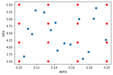
The Latin Hypercube design of experiments is advantageous over a factorial or grid-based design, as every experimental observation can provide useful information, even when some input factors are potentially unimportant or spurious.

As an example, consider the illustration below: 16 experiments are designed, either by making an evenly spaced grid over a two dimensional design space (i.e. a “full factorial” design) or by making the same number of latin hypercube draws.

import itertools
factorial = pd.DataFrame(
    itertools.product(np.linspace(*design.scope['alpha'].range, 4),
                      np.linspace(*design.scope['beta'].range, 4)),
    columns=['alpha', 'beta']
)
lhs = design_experiments(scope, n_samples=16, random_seed=4)

ax = factorial.plot.scatter('alpha', 'beta', color='r', s=40)
lhs.plot.scatter('alpha', 'beta', marker='s', s=40, ax=ax);

If it turns out that the “beta” input is not particularly important for some model outputs, the information we are actually getting on those outputs will have been derived from inputs that look like this:

factorial['beta'] = 0
lhs['beta'] = 1
ax = factorial.plot.scatter('alpha', 'beta', color='r', s=40, figsize=(6,1))
lhs.plot.scatter('alpha', 'beta', marker='s', s=40, ax=ax)
ax.set_ylim(-1,2)
ax.set_ylabel('')
ax.set_yticks([]);

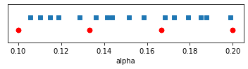
Essentially only four unique experiments remain under the full factorial design, while the Latin hypercube design still offers useful variance over all 16 experiments.

As for the sensitivity tests, the return type for the design_experiments function is emat.ExperimentalDesign. The result can be manipulated, saved, or reloaded as any other pandas DataFrame, which allows the the modeler to review an experimental design before actually running experiments.

lhs

	alpha	amortization_period	beta	debt_type	expand_capacity	input_flow	interest_rate	interest_rate_lock	unit_cost_expansion	value_of_time	yield_curve	free_flow_time	initial_capacity
0	0.179365	24	1	GO Bond	80.162643	120	0.034792	False	140.962953	0.049228	0.007397	60	100
1	0.105645	33	1	GO Bond	64.671571	126	0.030968	False	107.579380	0.137505	0.013873	60	100
2	0.141456	40	1	GO Bond	87.868001	131	0.033288	True	104.801110	0.065576	0.012420	60	100
3	0.118782	26	1	Rev Bond	16.323886	104	0.037495	False	134.207518	0.097838	0.004853	60	100
4	0.128577	29	1	GO Bond	94.525091	146	0.038427	True	117.693257	0.107705	0.016380	60	100
5	0.158509	42	1	Paygo	54.747060	115	0.034314	True	142.451442	0.027920	0.010428	60	100
6	0.172526	36	1	Rev Bond	11.215146	139	0.037112	True	110.962472	0.063330	0.001749	60	100
7	0.114949	32	1	Paygo	83.803917	148	0.036221	False	126.533101	0.083207	0.015196	60	100
8	0.198825	47	1	Paygo	37.148734	88	0.030445	True	115.398483	0.092398	-0.001874	60	100
9	0.185078	19	1	Rev Bond	1.086124	108	0.025081	True	95.638473	0.044881	0.000090	60	100
10	0.151665	50	1	Rev Bond	24.641162	99	0.028835	True	136.540190	0.124668	0.006217	60	100
11	0.110274	15	1	Rev Bond	71.659310	92	0.032085	False	104.141210	0.169572	0.019213	60	100
12	0.136319	18	1	Rev Bond	29.768710	83	0.028615	True	98.688980	0.150877	0.004064	60	100
13	0.143869	45	1	GO Bond	60.955126	133	0.026766	False	125.126753	0.079968	0.008846	60	100
14	0.187749	37	1	Paygo	49.882562	96	0.039660	False	129.689219	0.114333	0.017687	60	100
15	0.168406	22	1	Paygo	43.582987	118	0.027771	False	121.363034	0.018184	0.001277	60	100

In addition to the default Latin Hypercube sampler, TMIP-EMAT also includes several other samplers, which can be invoked through the sampler argument of the design_experiments function:

• 'ulhs' is a “uniform” latin hypercube sampler, which ignores all defined distribution shapes and correlations from the scope, instead using independent uniform distributions for all inputs. This sampler is useful when designing experiments to support a meta-model for a risk analysis that includes well characterized non-uniform uncertainties and correlations.
• 'mc' is a simple Monte Carlo sampler, which does not make attempts to ensure good coverage of the sampling space. This sampler minimizes overhead and is useful when running a very large number of simulations

Reference Designs

An additional convenience tool is included in TMIP-EMAT to create a “reference” design, which contains only a single experiment that has every input set at the default value. Although this one experiment is also included in the univariate sensitivity test design, an analyst may not need or want to run that full design. Having the reference case available can be helpful to add context to some exploratory visualizations.

from emat.experiment.experimental_design import design_refpoint_test
design_refpoint_test(scope)

	free_flow_time	initial_capacity	alpha	beta	input_flow	value_of_time	unit_cost_expansion	interest_rate	yield_curve	expand_capacity	amortization_period	debt_type	interest_rate_lock
0	60	100	0.15	4.0	100	0.075	100	0.03	0.01	10.0	30	GO Bond	False

Experimental Design API

emat.experiment.experimental_design.design_experiments(scope, n_samples_per_factor=10, n_samples=None, random_seed=1234, db=None, design_name=None, sampler='lhs', sample_from='all', jointly=True, redraws=1)

Create a design of experiments based on a Scope.

Parameters:

• scope (Scope) – The exploratory scope to use for the design.
• n_samples_per_factor (int, default 10) – The number of samples to draw per input factor in the design. To support the estimation of a meta-model, leaving this value at the default of 10 is generally a good plan; 10 draws per dimension will usually be sufficient for reasonably well behaved performance measure outputs, and if it is not sufficient then the number of draws that would be needed for good results is probably too many to be feasible.
• n_samples (int or tuple, optional) – The total number of samples in the design. If jointly is False, this is the number of samples in each of the uncertainties and the levers, the total number of samples will be the square of this value. Give a 2-tuple to set values for uncertainties and levers respectively, to set them independently. If this argument is given, it overrides n_samples_per_factor.
• random_seed (int or None, default 1234) – A random seed for reproducibility.
• db (Database, optional) – If provided, the generated design will be stored in the database indicated.
• design_name (str, optional) – A name for this design, to identify it in the database. If not given, a unique name will be generated based on the selected sampler.
• sampler (str or AbstractSampler, default ‘lhs’) –

  The sampler to use for this design. Available pre-defined samplers include:

  • ’lhs’: Latin Hypercube sampling
  • ’ulhs’: Uniform Latin Hypercube sampling, which ignores defined distribution shapes from the scope and samples everything as if it was from a uniform distribution
  • ’mc’: Monte carlo sampling, where independent random draws are made across all draws. This design has weaker space-covering properties than the LHS sampler, but may be appropriate for risk analysis and other large applications where coverage is not an issue.
  • ’uni’: Univariate sensitivity testing, whereby experiments are generated setting each parameter individually to minimum and maximum values (for numeric dtypes) or all possible values (for boolean and categorical dtypes). Note that designs for univariate sensitivity testing are deterministic and the number of samples given is ignored.
  • ’ref’: Reference point, which generates a design containing only a single experiment, with all parameters set at their default values.

• sample_from (‘all’, ‘uncertainties’, or ‘levers’) – The scope components from which to sample. The default is to sample from both uncertainties and levers, but it is also possible to sample only from one group of inputs or the other. Components not sampled are set at their default values in the design.
• jointly (bool, default True) – Whether to sample jointly all uncertainties and levers in a single design, or, if False, to generate separate samples for levers and uncertainties, and then combine the two in a full-factorial manner. This argument has no effect unless sample_from is ‘all’. Note that setting jointly to False may produce a very large design, as the total number of experiments will be the product of the number of experiments for the levers and the number of experiments for the uncertainties, which are set separately (i.e. if n_samples is given, the total number of experiments is the square of that value). Sampling jointly (the default) is appropriate for designing experiments to support the development of a meta-model. Sampling uncertainties and levers separately is appropriate for some other exploratory modeling applications, especially for directed search applications where the goal is to understand these two sets of input factors on their own.

Returns:

The resulting design. This is a specialized sub-class of a regular pandas.DataFrame, which attaches some useful meta-data to the DataFrame, including design_name, sampler_name, and scope.

Return type:

emat.experiment.ExperimentalDesign

emat.experiment.experimental_design.design_sensitivity_tests(scope, db=None, design_name='uni')

Create a design of univariate sensitivity tests based on a Scope.

If any of the parameters or levers have an infinite lower or upper bound, the sensitivity test will be made at the 1st or 99th percentile value respectively, instead of at the infinite value.

Parameters:

• scope (Scope) – The exploratory scope to use for the design.
• db (Database, optional) – If provided, this design will be stored in the database indicated.
• design_name (str, default ‘uni’) – A name for this design, primarily to identify it when stored in the database.

Returns:

The resulting design.

Return type:

emat.ExperimentalDesign

emat.experiment.experimental_design.design_refpoint_test(scope, db=None, design_name='ref')

Create a design containing a single reference point test based on a Scope.

Parameters:

• scope (Scope) – The exploratory scope to use for the design.
• db (Database, optional) – If provided, this design will be stored in the database indicated.
• design_name (str, default ‘ref’) – A name for this design, primarily to identify it when stored in the database.

Returns:

The resulting design.

Return type:

pandas.DataFrame