Database Walkthrough

import os
import numpy as np
import pandas as pd
import seaborn; seaborn.set_theme()
import plotly.io; plotly.io.templates.default = "seaborn"
import emat
import yaml
from emat.util.show_dir import show_dir
from emat.analysis import display_experiments
emat.versions()

emat 0.5.2, plotly 4.14.3

For this walkthrough of database features, we’ll work in a temporary directory. (In real projects you’ll likely want to save your data somewhere less ephemeral, so don’t just copy this tempfile code into your work.)

import tempfile
tempdir = tempfile.TemporaryDirectory()
os.chdir(tempdir.name)

We begin our example by populating a database with some experimental data, by creating and running a single design of experiments for the Road Test model.

import emat.examples
scope, db, model = emat.examples.road_test()
design = model.design_experiments()
model.run_experiments(design);

Single-Design Datasets

Writing Out Raw Data

When the database has only a single design of experiments, or if we don’t care about any differentiation between multiple designs that we may have created and ran, we can dump the entire set of model runs, including uncertainties, policy levers, and performance measures, all consolidated into a single pandas DataFrame using the read_experiment_all function. The constants even appear in this DataFrame too, for good measure.

df = db.read_experiment_all(scope.name)
df

	free_flow_time	initial_capacity	alpha	beta	input_flow	value_of_time	unit_cost_expansion	interest_rate	yield_curve	expand_capacity	amortization_period	debt_type	interest_rate_lock	no_build_travel_time	build_travel_time	time_savings	value_of_time_savings	net_benefits	cost_of_capacity_expansion	present_cost_expansion
experiment
1	60	100	0.184682	5.237143	115	0.059510	118.213466	0.031645	0.015659	18.224793	38	Rev Bond	False	83.038716	69.586789	13.451927	92.059972	-22.290905	114.350877	2154.415985
2	60	100	0.166133	4.121963	129	0.107772	141.322696	0.037612	0.007307	87.525790	36	Paygo	True	88.474313	62.132583	26.341730	366.219659	-16.843014	383.062672	12369.380535
3	60	100	0.198937	4.719838	105	0.040879	97.783320	0.028445	-0.001545	45.698048	44	GO Bond	False	75.027180	62.543328	12.483852	53.584943	-113.988412	167.573355	4468.506839
4	60	100	0.158758	4.915816	113	0.182517	127.224901	0.036234	0.004342	51.297546	42	GO Bond	True	77.370428	62.268768	15.101660	311.462907	11.539561	299.923347	6526.325171
5	60	100	0.157671	3.845952	133	0.067102	107.820482	0.039257	0.001558	22.824149	42	Paygo	False	88.328990	72.848428	15.480561	138.156464	78.036616	60.119848	2460.910705
...	...	...	...	...	...	...	...	...	...	...	...	...	...	...	...	...	...	...	...	...
106	60	100	0.169674	4.939898	150	0.131775	112.348054	0.033034	-0.000120	24.215074	34	Rev Bond	True	135.446332	85.847986	49.598345	980.371960	841.462782	138.909178	2720.516457
107	60	100	0.148297	3.824779	110	0.103255	105.248708	0.033437	0.007041	38.013885	22	GO Bond	True	72.811506	63.736168	9.075338	103.078214	-146.712793	249.791007	4000.912327
108	60	100	0.134701	3.627795	144	0.035233	132.063099	0.036702	0.018681	52.155613	32	Paygo	True	90.340993	66.617994	23.722999	120.358653	-112.568104	232.926757	6887.831931
109	60	100	0.176125	4.243675	100	0.188515	97.503468	0.035896	0.016807	38.352260	33	Paygo	True	70.567477	62.664842	7.902635	148.976184	25.480553	123.495631	3739.478399
110	60	100	0.142843	4.486119	145	0.064909	99.837764	0.035372	0.011055	15.851006	46	GO Bond	False	105.386378	83.456509	21.929869	206.401068	127.311542	79.089526	1582.528991

110 rows × 20 columns

Exporting this data is simply a matter of using the usual pandas methods to save the dataframe to a format of your choosing. We’ll save our data into a gzipped CSV file, which is somewhat compressed (we’re not monsters here) but still widely compatible for a variety of uses.

df.to_csv("road_test_1.csv.gz")

This table contains most of the information we want to export from our database, but not everything. We also probably want to have access to all of the information in the exploratory scope as well. Our example generator gives us a Scope reference directly, but if we didn’t have that we can still extract it from the database, using the read_scope method.

s = db.read_scope()
s

<emat.Scope with 2 constants, 7 uncertainties, 4 levers, 7 measures>

s.dump(filename="road_test_scope.yaml")

show_dir('.')

/
├── road_test_1.csv.gz
└── road_test_scope.yaml

Reading In Raw Data

Now, we’re ready to begin anew, constructing a fresh database from scratch, using only the raw formatted files.

First, let’s load our scope from the yaml file, and initialize a clean database using that scope.

s2 = emat.Scope("road_test_scope.yaml")

db2 = emat.SQLiteDB("road_test_2.sqldb")

db2.store_scope(s2)

Just as we used pandas to save out our consolidated DataFrame of experimental results, we can use it to read in a consolidated table of experiments.

df2 = pd.read_csv("road_test_1.csv.gz", index_col='experiment')
df2

	free_flow_time	initial_capacity	alpha	beta	input_flow	value_of_time	unit_cost_expansion	interest_rate	yield_curve	expand_capacity	amortization_period	debt_type	interest_rate_lock	no_build_travel_time	build_travel_time	time_savings	value_of_time_savings	net_benefits	cost_of_capacity_expansion	present_cost_expansion
experiment
1	60	100	0.184682	5.237143	115	0.059510	118.213466	0.031645	0.015659	18.224793	38	Rev Bond	False	83.038716	69.586789	13.451927	92.059972	-22.290905	114.350877	2154.415985
2	60	100	0.166133	4.121963	129	0.107772	141.322696	0.037612	0.007307	87.525790	36	Paygo	True	88.474313	62.132583	26.341730	366.219659	-16.843014	383.062672	12369.380535
3	60	100	0.198937	4.719838	105	0.040879	97.783320	0.028445	-0.001545	45.698048	44	GO Bond	False	75.027180	62.543328	12.483852	53.584943	-113.988412	167.573355	4468.506839
4	60	100	0.158758	4.915816	113	0.182517	127.224901	0.036234	0.004342	51.297546	42	GO Bond	True	77.370428	62.268768	15.101660	311.462907	11.539561	299.923347	6526.325171
5	60	100	0.157671	3.845952	133	0.067102	107.820482	0.039257	0.001558	22.824149	42	Paygo	False	88.328990	72.848428	15.480561	138.156464	78.036616	60.119848	2460.910705
...	...	...	...	...	...	...	...	...	...	...	...	...	...	...	...	...	...	...	...	...
106	60	100	0.169674	4.939898	150	0.131775	112.348054	0.033034	-0.000120	24.215074	34	Rev Bond	True	135.446332	85.847986	49.598345	980.371960	841.462782	138.909178	2720.516457
107	60	100	0.148297	3.824779	110	0.103255	105.248708	0.033437	0.007041	38.013885	22	GO Bond	True	72.811506	63.736168	9.075338	103.078214	-146.712793	249.791007	4000.912327
108	60	100	0.134701	3.627795	144	0.035233	132.063099	0.036702	0.018681	52.155613	32	Paygo	True	90.340993	66.617994	23.722999	120.358653	-112.568104	232.926757	6887.831931
109	60	100	0.176125	4.243675	100	0.188515	97.503468	0.035896	0.016807	38.352260	33	Paygo	True	70.567477	62.664842	7.902635	148.976184	25.480553	123.495631	3739.478399
110	60	100	0.142843	4.486119	145	0.064909	99.837764	0.035372	0.011055	15.851006	46	GO Bond	False	105.386378	83.456509	21.929869	206.401068	127.311542	79.089526	1582.528991

110 rows × 20 columns

Writing experiments to a database is not quite as simple as reading them. There is a parallel write_experiment_all method for the Database class, but to use it we need to provide not only the DataFrame of actual results, but also a name for the design of experiments we are writing (all experiments exist within designs) and the source of the performance measure results (zero means actual results from a core model run, and non-zero values are ID numbers for metamodels). This allows many different possible sets of performance measures to be stored for the same set of input parameters.

db2.write_experiment_all(
    scope_name=s2.name,
    design_name='general',
    source=0,
    xlm_df=df2,
)

display_experiments(s2, 'general', db=db2, rows=['time_savings'])

Time Savings

Multiple-Design Datasets

The EMAT database is not limited to storing a single design of experiments. Multiple designs can be stored for the same scope. We’ll add a set of univariate sensitivity test to our database, and a “ref” design that contains a single experiment with all inputs set to their default values.

design_uni = model.design_experiments(sampler='uni')
model.run_experiments(design_uni)
model.run_reference_experiment();

We now have three designs stored in our database. We can confirm this by reading out the set of design names.

db.read_design_names(s.name)

['lhs', 'ref', 'uni']

The design names we se here are the default names given when designs are created with each of the given samplers. When creating new designs, we can override the default names with other names of our choice using the design_name argument. The names can be any string not already in use.

design_b = model.design_experiments(sampler='lhs', design_name='bruce')
db.read_design_names(s.name)

['bruce', 'lhs', 'ref', 'uni']

If you try to re-use a name you’ll get an error, as having multiple designs with the same name does not allow you to make it clear which design you are referring to.

try:
    model.design_experiments(sampler='lhs', design_name='bruce')
except ValueError as err:
    print(err)

the design "bruce" already exists for scope "EMAT Road Test"

As noted above, the design name, which can be any string, is separate from the sampler method. A default design name based on the name of the sampler method is used if no design name is given. The selected sampler must be one available in EMAT, as the sampler defines a particular logic about how to generate the design.

try:
    model.design_experiments(sampler='uni')
except ValueError as err:
    print(err)

Note that there can be some experiments that are in more than one design. This is not merely duplicating the experiment and results, but actually assigning the same experiment to both designs. We can see this for the ‘uni’ and ‘ref’ designs – both contain the all-default parameters experiment, and when we read these designs out of the database, the same experiment number is reported out in both designs.

db.read_experiment_all(scope.name, design_name='uni').head()

	free_flow_time	initial_capacity	alpha	beta	input_flow	value_of_time	unit_cost_expansion	interest_rate	yield_curve	expand_capacity	amortization_period	debt_type	interest_rate_lock	no_build_travel_time	build_travel_time	time_savings	value_of_time_savings	net_benefits	cost_of_capacity_expansion	present_cost_expansion
experiment
111	60	100	0.15	4.0	100	0.075	100.0	0.03	0.01	10.0	30	GO Bond	False	69.0	66.147121	2.852879	21.396592	-30.807346	52.203937	1000.0
112	60	100	0.10	4.0	100	0.075	100.0	0.03	0.01	10.0	30	GO Bond	False	66.0	64.098081	1.901919	14.264395	-37.939543	52.203937	1000.0
113	60	100	0.20	4.0	100	0.075	100.0	0.03	0.01	10.0	30	GO Bond	False	72.0	68.196161	3.803839	28.528789	-23.675148	52.203937	1000.0
114	60	100	0.15	3.5	100	0.075	100.0	0.03	0.01	10.0	30	GO Bond	False	69.0	66.447155	2.552845	19.146338	-33.057600	52.203937	1000.0
115	60	100	0.15	5.5	100	0.075	100.0	0.03	0.01	10.0	30	GO Bond	False	69.0	65.328227	3.671773	27.538295	-24.665642	52.203937	1000.0

db.read_experiment_all(scope.name, design_name='ref')

	free_flow_time	initial_capacity	alpha	beta	input_flow	value_of_time	unit_cost_expansion	interest_rate	yield_curve	expand_capacity	amortization_period	debt_type	interest_rate_lock	no_build_travel_time	build_travel_time	time_savings	value_of_time_savings	net_benefits	cost_of_capacity_expansion	present_cost_expansion
experiment
111	60	100	0.15	4.0	100	0.075	100.0	0.03	0.01	10.0	30	GO Bond	False	69.0	66.147121	2.852879	21.396592	-30.807346	52.203937	1000.0

One “gotcha” to be wary of is unintentionally replicating experiments. By default, the random_seed for randomly generated experiemnts is set to 0 for reproducibility. This means that, for example, the ‘bruce’ design is actually the same as the original ‘lhs’ design:

db.read_experiment_all(scope.name, design_name='lhs').equals(
    db.read_experiment_all(scope.name, design_name='bruce')
)

True

If we want a new set of random experiments with the same sampler and other parameters, we’ll need to provide a different random_seed.

design_b = model.design_experiments(sampler='lhs', design_name='new_bruce', random_seed=42)
db.read_experiment_all(scope.name, design_name='lhs').equals(design_b)

False

Writing Out Raw Data

We can read a single dataframe containing all the experiments associated with this scope by omitting the design_name argument, just as if there was only one design.

df = db.read_experiment_all(scope.name)
df

	free_flow_time	initial_capacity	alpha	beta	input_flow	value_of_time	unit_cost_expansion	interest_rate	yield_curve	expand_capacity	amortization_period	debt_type	interest_rate_lock	no_build_travel_time	build_travel_time	time_savings	value_of_time_savings	net_benefits	cost_of_capacity_expansion	present_cost_expansion
experiment
1	60	100	0.184682	5.237143	115	0.059510	118.213466	0.031645	0.015659	18.224793	38	Rev Bond	False	83.038716	69.586789	13.451927	92.059972	-22.290905	114.350877	2154.415985
2	60	100	0.166133	4.121963	129	0.107772	141.322696	0.037612	0.007307	87.525790	36	Paygo	True	88.474313	62.132583	26.341730	366.219659	-16.843014	383.062672	12369.380535
3	60	100	0.198937	4.719838	105	0.040879	97.783320	0.028445	-0.001545	45.698048	44	GO Bond	False	75.027180	62.543328	12.483852	53.584943	-113.988412	167.573355	4468.506839
4	60	100	0.158758	4.915816	113	0.182517	127.224901	0.036234	0.004342	51.297546	42	GO Bond	True	77.370428	62.268768	15.101660	311.462907	11.539561	299.923347	6526.325171
5	60	100	0.157671	3.845952	133	0.067102	107.820482	0.039257	0.001558	22.824149	42	Paygo	False	88.328990	72.848428	15.480561	138.156464	78.036616	60.119848	2460.910705
...	...	...	...	...	...	...	...	...	...	...	...	...	...	...	...	...	...	...	...	...
238	60	100	0.164649	4.851786	104	0.012456	127.667298	0.025673	0.012674	24.114264	30	GO Bond	True	NaN	NaN	NaN	NaN	NaN	NaN	NaN
239	60	100	0.113568	4.545709	105	0.137105	139.911784	0.028280	0.016936	92.883345	15	GO Bond	True	NaN	NaN	NaN	NaN	NaN	NaN	NaN
240	60	100	0.184434	4.732430	144	0.100242	99.904559	0.030392	0.019534	84.793007	15	GO Bond	True	NaN	NaN	NaN	NaN	NaN	NaN	NaN
241	60	100	0.146598	3.616301	107	0.065130	135.593036	0.035733	0.002085	29.107628	34	Paygo	True	NaN	NaN	NaN	NaN	NaN	NaN	NaN
242	60	100	0.193327	5.402220	134	0.048285	140.945872	0.026210	-0.001255	26.285726	44	Rev Bond	False	NaN	NaN	NaN	NaN	NaN	NaN	NaN

242 rows × 20 columns

This dataframe is different than the one we saw earlier with the same command, as we have since added a few more experiments to the database in a few different designs. If we don’t give a design_name argument, we’ll retrieve every (unique) experiment from every design currently stored in the database.

df.to_csv("road_test_2.csv.gz")

If we want to be able to reconstruct the various designs of experiments later, we’ll also need to write out instructions for that. The read_all_experiment_ids method can give us a dictionary of all the relevant information.

design_experiments = db.read_all_experiment_ids(scope.name, design_name='*',grouped=True)
design_experiments

{'bruce': '1-110',
 'lhs': '1-110',
 'new_bruce': '133-242',
 'ref': '111',
 'uni': '111-132',
 'uni_2': '111-132'}

We can write this dictionary to a file in ‘yaml’ format.

with open("road_test_design_experiments.yaml", 'wt') as f:
    yaml.dump(design_experiments, f)

Reading In Raw Data

To construct a new emat Database with multiple designs of experients,…

db3 = emat.SQLiteDB("road_test_3.sqldb")
db3.store_scope(s2)

df3 = pd.read_csv("road_test_2.csv.gz", index_col='experiment')
df3

	free_flow_time	initial_capacity	alpha	beta	input_flow	value_of_time	unit_cost_expansion	interest_rate	yield_curve	expand_capacity	amortization_period	debt_type	interest_rate_lock	no_build_travel_time	build_travel_time	time_savings	value_of_time_savings	net_benefits	cost_of_capacity_expansion	present_cost_expansion
experiment
1	60	100	0.184682	5.237143	115	0.059510	118.213466	0.031645	0.015659	18.224793	38	Rev Bond	False	83.038716	69.586789	13.451927	92.059972	-22.290905	114.350877	2154.415985
2	60	100	0.166133	4.121963	129	0.107772	141.322696	0.037612	0.007307	87.525790	36	Paygo	True	88.474313	62.132583	26.341730	366.219659	-16.843014	383.062672	12369.380535
3	60	100	0.198937	4.719838	105	0.040879	97.783320	0.028445	-0.001545	45.698048	44	GO Bond	False	75.027180	62.543328	12.483852	53.584943	-113.988412	167.573355	4468.506839
4	60	100	0.158758	4.915816	113	0.182517	127.224901	0.036234	0.004342	51.297546	42	GO Bond	True	77.370428	62.268768	15.101660	311.462907	11.539561	299.923347	6526.325171
5	60	100	0.157671	3.845952	133	0.067102	107.820482	0.039257	0.001558	22.824149	42	Paygo	False	88.328990	72.848428	15.480561	138.156464	78.036616	60.119848	2460.910705
...	...	...	...	...	...	...	...	...	...	...	...	...	...	...	...	...	...	...	...	...
238	60	100	0.164649	4.851786	104	0.012456	127.667298	0.025673	0.012674	24.114264	30	GO Bond	True	NaN	NaN	NaN	NaN	NaN	NaN	NaN
239	60	100	0.113568	4.545709	105	0.137105	139.911784	0.028280	0.016936	92.883345	15	GO Bond	True	NaN	NaN	NaN	NaN	NaN	NaN	NaN
240	60	100	0.184434	4.732430	144	0.100242	99.904559	0.030392	0.019534	84.793007	15	GO Bond	True	NaN	NaN	NaN	NaN	NaN	NaN	NaN
241	60	100	0.146598	3.616301	107	0.065130	135.593036	0.035733	0.002085	29.107628	34	Paygo	True	NaN	NaN	NaN	NaN	NaN	NaN	NaN
242	60	100	0.193327	5.402220	134	0.048285	140.945872	0.026210	-0.001255	26.285726	44	Rev Bond	False	NaN	NaN	NaN	NaN	NaN	NaN	NaN

242 rows × 20 columns

with open("road_test_design_experiments.yaml", 'rt') as f:
    design_experiments2 = yaml.safe_load(f)
design_experiments2

{'bruce': '1-110',
 'lhs': '1-110',
 'new_bruce': '133-242',
 'ref': '111',
 'uni': '111-132',
 'uni_2': '111-132'}

db3.write_experiment_all(
    scope_name=s2.name,
    design_name=design_experiments2,
    source=0,
    xlm_df=df3,
)

db3.read_design_names(s.name)

['bruce', 'lhs', 'new_bruce', 'ref', 'uni', 'uni_2']

db3.read_all_experiment_ids(scope.name, design_name='*',grouped=True)

{'bruce': '1-110',
 'lhs': '1-110',
 'new_bruce': '133-242',
 'ref': '111',
 'uni': '111-132',
 'uni_2': '111-132'}

db3.read_experiment_all(scope.name, design_name='uni').head()

	free_flow_time	initial_capacity	alpha	beta	input_flow	value_of_time	unit_cost_expansion	interest_rate	yield_curve	expand_capacity	amortization_period	debt_type	interest_rate_lock	no_build_travel_time	build_travel_time	time_savings	value_of_time_savings	net_benefits	cost_of_capacity_expansion	present_cost_expansion
experiment
111	60	100	0.15	4.0	100	0.075	100.0	0.03	0.01	10.0	30	GO Bond	False	69.0	66.147121	2.852879	21.396592	-30.807346	52.203937	1000.0
112	60	100	0.10	4.0	100	0.075	100.0	0.03	0.01	10.0	30	GO Bond	False	66.0	64.098081	1.901919	14.264395	-37.939543	52.203937	1000.0
113	60	100	0.20	4.0	100	0.075	100.0	0.03	0.01	10.0	30	GO Bond	False	72.0	68.196161	3.803839	28.528789	-23.675148	52.203937	1000.0
114	60	100	0.15	3.5	100	0.075	100.0	0.03	0.01	10.0	30	GO Bond	False	69.0	66.447155	2.552845	19.146338	-33.057600	52.203937	1000.0
115	60	100	0.15	5.5	100	0.075	100.0	0.03	0.01	10.0	30	GO Bond	False	69.0	65.328227	3.671773	27.538295	-24.665642	52.203937	1000.0

Re-running Experiments

This section provides a short walkthrough of how to handle mistakes in an EMAT database. By “mistakes” we are referring to incorrect values that have been written into the database by accident, generally arising from core model runs that were misconfigured or suffered non-fatal errors that caused the results to be invalid.

One approach to handling such problems is to simply start over with a brand new clean database file. However, this may be inconvenient if the database already includes a number of valid results, especially if those valid results were expensive to generate. It may also be desirable to keep prior invalid results on hand, so as to easily recognized when errors recur.

We begin this example by populating our database with some more experimental data, by creating and running a single design of experiments for the Road Test model, except these experiments will be created with a misconfigured model (lane_width = 11, it should be 10), so the results will be bad. (In general, you probably won’t intentionally create corrupt data, but we’re doing so here for expository purposes, so we’ll give this design a name of ‘oops’ so we can readily recall what we’ve done.)

model.lane_width = 10.3
oops = model.design_experiments(design_name='oops', random_seed=12345)
model.run_experiments(oops);

We can review a dataframe of results as before, using the read_experiment_all method. This time we will add with_run_ids=True, which will add an extra column to the index, showing a universally unique id attached to each row of results.

oops_result1 = db.read_experiment_all(scope.name, 'oops', with_run_ids=True)
oops_result1.head()

		free_flow_time	initial_capacity	alpha	beta	input_flow	value_of_time	unit_cost_expansion	interest_rate	yield_curve	expand_capacity	amortization_period	debt_type	interest_rate_lock	no_build_travel_time	build_travel_time	time_savings	value_of_time_savings	net_benefits	cost_of_capacity_expansion	present_cost_expansion
experiment	run
243	b2358b5e-be73-11eb-809d-acde48001122	60	100	0.157955	4.270404	112	0.151487	116.445987	0.029784	0.018968	50.163393	38	Rev Bond	False	75.376818	79.495869	-4.119051	-69.886026	-381.303111	311.417085	5841.325841
244	b2376db6-be73-11eb-809d-acde48001122	60	100	0.165144	4.008218	134	0.039670	102.879244	0.032505	0.000708	57.330143	40	Rev Bond	False	92.024075	83.059349	8.964726	47.654780	-220.075486	267.730266	5898.081794
245	b238ff32-be73-11eb-809d-acde48001122	60	100	0.103964	4.019636	92	0.100936	131.282035	0.038432	0.002658	64.949710	39	GO Bond	True	64.461446	77.449591	-12.988145	-120.608948	-520.723349	400.114402	8526.730135
246	b23a6b42-be73-11eb-809d-acde48001122	60	100	0.172162	4.920619	144	0.135484	95.348634	0.025803	0.008870	77.498534	26	Paygo	False	122.134147	80.716842	41.417305	808.041389	513.014691	295.026699	7389.379292
247	b23bdc66-be73-11eb-809d-acde48001122	60	100	0.136954	4.901048	100	0.109919	114.310247	0.027538	0.016733	46.312847	41	Paygo	False	68.217253	78.289223	-10.071970	-110.710261	-276.303370	165.593109	5294.033017

display_experiments(scope, oops_result1, rows=['time_savings'])

Time Savings

Some of these results are obviously problematic. Increasing capacity cannot possibly result in a negative travel time savings. (Braess paradox doesn’t apply here because it’s just one link, not a network.) So those negative values are clearly wrong. We can fix the model so they won’t be wrong, but by default the run_experiments method won’t actually re-run models when the results are already available in the database. To solve this conundrum, we can mark the incorrect results as invalid, using a query to pull out the rows that can be flagged as wrong.

db.invalidate_experiment_runs(
    queries=['time_savings < 0']
)

[73]

The [73] returned here indicates that 73 sets of results were invalidated by this command. The invalidation command actually sets a “valid” flag in the database to False for these experiment runs, so that a persistant record that they are bad is stored in the database. Now we can fix our model, and then use the run_experiments method to get new model runs for the invalidated results.

model.lane_width = 10
oops_result2 = model.run_experiments(oops)

display_experiments(scope, 'oops', db=db, rows=['time_savings'])

Time Savings

The re-run fixed the negative values, although it left in place the other experimental runs in the database. By the way we constructed this example, we know those are wrong too, and it’s evident in the apparent discontinuity in the input flow graph, which we can zoom in on.

ax = oops_result2.plot.scatter(x='input_flow', y='time_savings', color='r')
ax.plot([109,135], [0,35], '--',color='y');

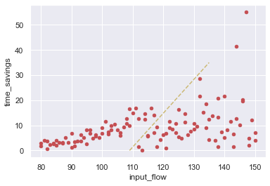
Those original results are bad too, and we want to invalidate them as well. In addition to giving conditional queries to the invalidate_experiment_runs method, we can also give a dataframe of results that have run ids attached, and those unique ids will be used to to find and invalidate results in the database. Here, we pass in the dataframe of all the results, which contains all 110 runs, but only 37 runs are newly invalidated (77 were invalidated previously).

db.invalidate_experiment_runs(
    oops_result1
)

37

Now when we run the experiments again, those 37 experiments are re-run.

oops_result3 = model.run_experiments(oops)

display_experiments(scope, 'lhs', db=db, rows=['time_savings'])

Time Savings

Writing Out All Runs

By default, the read_experiment_all method returns the most recent valid set of performance measures for each experiment, but we can override this behavior to ask for 'all' run results, or all 'valid' or 'invalid' results, by setting the runs argument to those literal values. This allows us to easily write out data files containing all the results stored in the database.

db.read_experiment_all(scope.name, with_run_ids=True, runs='all')

		free_flow_time	initial_capacity	alpha	beta	input_flow	value_of_time	unit_cost_expansion	interest_rate	yield_curve	expand_capacity	amortization_period	debt_type	interest_rate_lock	no_build_travel_time	build_travel_time	time_savings	value_of_time_savings	net_benefits	cost_of_capacity_expansion	present_cost_expansion
experiment	run
1	af00ae82-be73-11eb-809d-acde48001122	60	100	0.184682	5.237143	115	0.059510	118.213466	0.031645	0.015659	18.224793	38	Rev Bond	False	83.038716	69.586789	13.451927	92.059972	-22.290905	114.350877	2154.415985
2	af0320e0-be73-11eb-809d-acde48001122	60	100	0.166133	4.121963	129	0.107772	141.322696	0.037612	0.007307	87.525790	36	Paygo	True	88.474313	62.132583	26.341730	366.219659	-16.843014	383.062672	12369.380535
3	af04aaaa-be73-11eb-809d-acde48001122	60	100	0.198937	4.719838	105	0.040879	97.783320	0.028445	-0.001545	45.698048	44	GO Bond	False	75.027180	62.543328	12.483852	53.584943	-113.988412	167.573355	4468.506839
4	af0628e4-be73-11eb-809d-acde48001122	60	100	0.158758	4.915816	113	0.182517	127.224901	0.036234	0.004342	51.297546	42	GO Bond	True	77.370428	62.268768	15.101660	311.462907	11.539561	299.923347	6526.325171
5	af07aea8-be73-11eb-809d-acde48001122	60	100	0.157671	3.845952	133	0.067102	107.820482	0.039257	0.001558	22.824149	42	Paygo	False	88.328990	72.848428	15.480561	138.156464	78.036616	60.119848	2460.910705
...	...	...	...	...	...	...	...	...	...	...	...	...	...	...	...	...	...	...	...	...	...
350	b3f00848-be73-11eb-809d-acde48001122	60	100	0.127109	4.855843	103	0.130109	110.140882	0.039189	0.016098	69.050648	31	GO Bond	False	68.803652	60.687779	8.115873	108.762921	-345.671302	454.434223	7605.299268
351	b2d23300-be73-11eb-809d-acde48001122	60	100	0.191902	4.144514	102	0.145524	141.761624	0.037483	0.004611	20.006234	45	GO Bond	True	72.499003	83.787080	-11.288077	-167.553833	-295.911196	128.357363	2836.116224
	b3f17d7c-be73-11eb-809d-acde48001122	60	100	0.191902	4.144514	102	0.145524	141.761624	0.037483	0.004611	20.006234	45	GO Bond	True	72.499003	65.869676	6.629328	98.401992	-29.955371	128.357363	2836.116224
352	b2d3b568-be73-11eb-809d-acde48001122	60	100	0.189252	4.588903	111	0.191116	105.423753	0.038912	0.012596	70.999408	16	Rev Bond	True	78.330479	78.364867	-0.034388	-0.729512	-597.920964	597.191453	7485.024087
	b3f2fdd2-be73-11eb-809d-acde48001122	60	100	0.189252	4.588903	111	0.191116	105.423753	0.038912	0.012596	70.999408	16	Rev Bond	True	78.330479	61.563090	16.767389	355.700934	-241.490519	597.191453	7485.024087

462 rows × 20 columns

In the resulting dataframe above, we can see that we have retrieved two different runs for some of the experiments. Only one of them is valid for each. If we want to get all the stored runs and also mark the valid and invalid runs, we can read them seperately and attach a tag to the two dataframes.

runs_1 = db.read_experiment_all(scope.name, with_run_ids=True, runs='valid')
runs_1['is_valid'] = True
runs_0 = db.read_experiment_all(scope.name, with_run_ids=True, runs='invalid', only_with_measures=True)
runs_0['is_valid'] = False
all_runs = pd.concat([runs_1, runs_0])
all_runs.sort_index()

		free_flow_time	initial_capacity	alpha	beta	input_flow	value_of_time	unit_cost_expansion	interest_rate	yield_curve	expand_capacity	...	debt_type	interest_rate_lock	no_build_travel_time	build_travel_time	time_savings	value_of_time_savings	net_benefits	cost_of_capacity_expansion	present_cost_expansion	is_valid
experiment	run
1	af00ae82-be73-11eb-809d-acde48001122	60	100	0.184682	5.237143	115	0.059510	118.213466	0.031645	0.015659	18.224793	...	Rev Bond	False	83.038716	69.586789	13.451927	92.059972	-22.290905	114.350877	2154.415985	True
2	af0320e0-be73-11eb-809d-acde48001122	60	100	0.166133	4.121963	129	0.107772	141.322696	0.037612	0.007307	87.525790	...	Paygo	True	88.474313	62.132583	26.341730	366.219659	-16.843014	383.062672	12369.380535	True
3	af04aaaa-be73-11eb-809d-acde48001122	60	100	0.198937	4.719838	105	0.040879	97.783320	0.028445	-0.001545	45.698048	...	GO Bond	False	75.027180	62.543328	12.483852	53.584943	-113.988412	167.573355	4468.506839	True
4	af0628e4-be73-11eb-809d-acde48001122	60	100	0.158758	4.915816	113	0.182517	127.224901	0.036234	0.004342	51.297546	...	GO Bond	True	77.370428	62.268768	15.101660	311.462907	11.539561	299.923347	6526.325171	True
5	af07aea8-be73-11eb-809d-acde48001122	60	100	0.157671	3.845952	133	0.067102	107.820482	0.039257	0.001558	22.824149	...	Paygo	False	88.328990	72.848428	15.480561	138.156464	78.036616	60.119848	2460.910705	True
...	...	...	...	...	...	...	...	...	...	...	...	...	...	...	...	...	...	...	...	...	...	...
350	b3f00848-be73-11eb-809d-acde48001122	60	100	0.127109	4.855843	103	0.130109	110.140882	0.039189	0.016098	69.050648	...	GO Bond	False	68.803652	60.687779	8.115873	108.762921	-345.671302	454.434223	7605.299268	True
351	b2d23300-be73-11eb-809d-acde48001122	60	100	0.191902	4.144514	102	0.145524	141.761624	0.037483	0.004611	20.006234	...	GO Bond	True	72.499003	83.787080	-11.288077	-167.553833	-295.911196	128.357363	2836.116224	False
	b3f17d7c-be73-11eb-809d-acde48001122	60	100	0.191902	4.144514	102	0.145524	141.761624	0.037483	0.004611	20.006234	...	GO Bond	True	72.499003	65.869676	6.629328	98.401992	-29.955371	128.357363	2836.116224	True
352	b2d3b568-be73-11eb-809d-acde48001122	60	100	0.189252	4.588903	111	0.191116	105.423753	0.038912	0.012596	70.999408	...	Rev Bond	True	78.330479	78.364867	-0.034388	-0.729512	-597.920964	597.191453	7485.024087	False
	b3f2fdd2-be73-11eb-809d-acde48001122	60	100	0.189252	4.588903	111	0.191116	105.423753	0.038912	0.012596	70.999408	...	Rev Bond	True	78.330479	61.563090	16.767389	355.700934	-241.490519	597.191453	7485.024087	True

462 rows × 21 columns

These mechanisms can be use to write out results of multiple runs, and to repopulate a database with both valid and invalid raw results. This can be done multiple ways (seperate files, one combined file, keeping track of invalidation queries, etc.). The particular implementations of each are left as an exercise for the reader.