import emat
emat.versions()

emat 0.5.2, plotly 4.14.3

PRIM

Patient rule induction method (PRIM) is a scenario discovery algorithm that operates on an existing set of data with model inputs and outputs (i.e., you have already designed and run a set of experiments using either a core model or a meta-model.) Generally, a decently size set of experiments (hundreds or thousands) is used to describe the solution space, although no minimum number of experiments is formally required.

PRIM is used for locating areas of an outcome space that are of particular interest, which it does by reducing the data size incrementally by small amounts in an iterative process as follows:

• Candidate boxes are generated. These boxes represent incrementally smaller sets of the data. Each box removes a portion of the data based on the levels of a single input variable.
  • For categorical input variables, there is one box generated for each category with each box removing one category from the data set.
  • For integer and continuous variables, two boxes are generated – one box that removes a portion of data representing the smallest set of values for that input variable and another box that removes a portion of data representing the largest set of values for that input. The step size for these variables is controlled by the analyst.
• For each candidate box, the relative improvement in the number of outcomes of interest inside the box is calculated and the candidate box with the highest improvement is selected.
• The data in the selected candidate box replaces the starting data and the process is repeated.

The process ends based on a stopping criteria. For more details on the algorithm, see Friedman and Fisher (1999) or Kwakkel and Jaxa-Rozen (2016).

The PRIM algorithm is particularly useful for scenario discovery, which broadly is the process of identifying particular scenarios of interest in a large and deeply uncertain dataset. In the context of exploratory modeling, scenario discovery is often used to obtain a better understanding of areas of the uncertainty space where a policy or collection of policies performs poorly because it is often used in tandem with robust search methods for identifying policies that perform well (Kwakkel and Jaxa-Rozen (2016)).

The Mechanics of using PRIM

In order to use PRIM for scenario discovery, the analyst must first conduct a set of experiments. This includes having both the inputs and outputs of the experiments (i.e., you’ve already run the model or meta-model).

import emat.examples
scope, db, model = emat.examples.road_test()
designed = model.design_experiments(n_samples=5000, sampler='mc', random_seed=42)
results = model.run_experiments(designed, db=False)

In order to use PRIM for scenario discovery, the analyst must also identify what constitutes a case that is “of interest”. This is essentially generating a True/False label for every case, using some combination of values of the output performance measures as well as (possibly) the values of the inputs. Some examples of possible definitions of “of interest” might include:

• Cases where total predicted VMT (a performance measure) is below some threshold.
• Cases where transit farebox revenue (a performance measure) is above some threshold.
• Cases where transit farebox revenue (a performance measure) is above above 50% of budgeted transit operating cost (a policy lever).
• Cases where the average speed of tolled lanes (a performance measure) is less than free-flow speed but greater than 85% of free-flow speed (i.e., bounded both from above and from below).
• Cases that meet all of the above criteria simultaneously.

The salient features of a definition for “of interest” is that (a) it can be calculated for each case if given the set of inputs and outputs, and (b) that the result is a True or False value.

For this example, we will define “of interest” as cases from the Road Test example that have positive net benefits.

of_interest = results['net_benefits']>0

Having defined the cases of interest, to use PRIM we pass the explanatory data (i.e., the inputs) and the ‘of_interest’ variable to the Prim object, and then invoke the find_box method.

from emat.analysis.prim import Prim

discovery = Prim(
    model.read_experiment_parameters(design_name='mc'),
    of_interest,
    threshold=0.02,
    scope=scope
)

box1 = discovery.find_box()

The find_box command actually provides a number of different possible boxes along a (heuristically) optimal trajectory, trading off coverage against density. We can plot a static figure showing the tradeoff curve using the show_tradeoff command:

ax = box1.show_tradeoff()

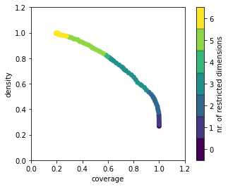
This figure shows the trade-off between coverage and density.

• Coverage is percentage of the cases of interest that are in the box (i.e., number of cases of interest in the box divided by total number of cases of interest). The starting point of the PRIM algorithm is the unrestricted full set of cases, which includes all outcomes of interest, and therefore, the coverage starts at 1.0 and drops as the algorithm progresses.
• Density is the share of cases in the box that are case of interest (i.e., number of cases of interest in the box divided by the total number of cases in the box). As the box is reduced, the density will increase (as that is the objective of the PRIM algorithm).

For the statistically minded, this tradeoff can also be interpreted as the tradeoff between Type I (false positive) and Type II (false negative) error. High coverage minimizes the false negatives, while high density minimizes false positives.

By default, the PRIM algorithm sets the “selected” box position as the particular box at the end of the peeling trajectory (highest density, at the top of the top of the tradeoff curve), which has the highest density, but the smallest coverage.

box1

<PrimBox peel 82 of 82>
   coverage: 0.21257
   density:  0.99649
   mean: 0.99649
   mass: 0.05700
   restricted dims: 6
                               min        max
     expand_capacity      0.004812  60.324206
     input_flow                125        150
     value_of_time        0.067766   0.238765
     beta                 4.505424    5.49961
     amortization_period        18         50
     alpha                 0.10917   0.198906

In a Jupyter notebook, the analyst can interactively view and select other possible boxes using the tradeoff_selector method. This method opens a dynamic viewer which shows the same basic figure as the static one above, but when hovering over each possible tradeoff point, a pop-up box appears with more details about that point, including which dimensions are restricted, and what the restrictions are. A selection of the preferred tradeoff can be made by clicking on any point.† The currently selected preferred tradeoff is marked with an “X” instead of a dot.

box1.tradeoff_selector()

In addition to the point-and-click interface, the analyst can also manually set the selection programmatically using Python code, selecting a preferred box (by index) that trades off density and coverage.

box1.select(30)
box1

<PrimBox peel 31 of 82>
   coverage: 0.72904
   density:  0.71043
   mean: 0.71043
   mass: 0.27420
   restricted dims: 3
                           min       max
     expand_capacity  0.004812  86.06928
     input_flow            116       150
     value_of_time    0.067171  0.238765

To help visualize these restricted dimensions better, we can generate a plot of the resulting box, overlaid on a ‘pairs’ scatter plot matrix (splom) of the various restricted dimensions.

In the figure below, each of the three restricted dimensions represents both a row and a column of figures. Each of the off-diagonal charts show bi-dimensional distribution of the data across two of the actively restricted dimensions. These charts are overlaid with a green rectangle denoting the selected box. The on-diagonal charts show the relative distribution of cases that are and are not of interest (unconditional on the selected box).

box1.splom()

Depending on the number of experiments in the data and the number and distribution of the cases of interest, it may be clearer to view these figures as a heat map matrix (hmm) intead of a splom.

box1.hmm()

Non-Rectangular Boxes

Regardless of any analyst intervention in box selection using the select method, initial box identified using PRIM will always be a rectangle (or, more generally, a hyper-rectangle). Every restricted dimension is specified independently, not conditional on any other dimension.

A second box can be overlaid after the first to expand the solution to include a non-rectangular area. The second tier box itself is still another rectangle, but it can be defined using different boundaries, possibly on different dimensions, to give in aggregate a non-convex shape. Creating such a second box is done by calling the find_box method again, after the particulars of the first box are finalized.

box2 = discovery.find_box()

box2

<PrimBox peel 48 of 48>
   coverage: 0.11751
   density:  0.43014
   mean: 0.43014
   mass: 0.07300
   restricted dims: 8
                                        min                max
     unit_cost_expansion          95.000837         142.588934
     expand_capacity               0.004812          97.595439
     input_flow                         112                150
     beta                          4.051416            5.49961
     value_of_time                 0.035604           0.238765
     amortization_period                 20                 50
     alpha                         0.110845           0.199972
     debt_type            {Rev Bond, Paygo}  {Rev Bond, Paygo}

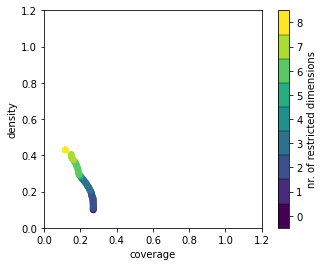
The cases considered for the second box are only those cases not within the first box. Because our first box had a relatively high coverage and high density, we have already captured most of the cases of interest and not too many other cases, so the second box has a much diminished trade-off curve. The maximum value of the coverage for this second box is one minus the selected final coverage of the first box.

box2.show_tradeoff();

We can also make a similar scatter plot for this second box. There are 8 restricted dimensions in the currently selected solution, which can result in an unwieldy large scatter plot matrix. To help, the splom command allows you to override the selection of dimensions to display in the rows and/or columns of the resulting figure, by explicitly giving a set of dimensions to display. These don’t necessarily need to be restricted dimensions, they can be any dimensions available in the original PRIM analysis.

Because this is the second box, the method will only plot the points that remain (i.e. the ones not included in the first box). This results in a “blotchy” appearance for may of the graphs in this figure, as most of the “of interest” cases were captured previously.

box2.splom(
    cols=['beta','input_flow','value_of_time','debt_type','yield_curve']
)

PRIM API

class emat.analysis.Prim(x, y, threshold=0.05, *args, scope=None, explorer=None, **kwargs)

Bases: emat.workbench.analysis.prim.Prim, emat.analysis.discovery.ScenarioDiscoveryMixin

Patient rule induction method

This implementation of Prim is derived from the EMA workbench, and is enhanced to work interactively within the TMIP-EMAT framework.

Parameters:

• x (pandas.DataFrame) – The independent variables, generally the scoped input parameters (uncertainties and/or policy levers) from a design of experiments.
• y (array-like) – The dependent variable, generally a pandas.Series or other one dimensional array with size equal to the number of rows in x.
• threshold (float) – The density threshold that a box must meet.
• obj_function ({LENIENT1, LENIENT2, ORIGINAL}) – The objective function used by PRIM. This defaults to a lenient objective function based on the gain of mean divided by the loss of mass.
• peel_alpha (float, default 0.05) – The parameter controlling the peeling stage.
• paste_alpha (float, default 0.05) – The parameter controlling the pasting stage.
• mass_min (float, default 0.05) – The minimum mass of a box.
• threshold_type ({ABOVE, BELOW}) – Whether to look above or below the threshold value.
• mode (RuleInductionType) – This PRIM implementation defaults to binary classification, but this argument can be used to switch to regression mode. In binary mode, the y array should only have binary values, while in regression mode it can contain other floating point values.
• update_function ({‘default’, ‘guivarch’}) – The default behavior for this algorithm after finding the first box is to remove all points in the first box, so that subsequent boxes do not include them. An alternate procedure suggested by Guivarch et al (2016) doi:10.1016/j.envsoft.2016.03.006 is to simply set all points in the first box to be no longer of interest. This alternate procedure is only valid in binary mode.

property boxes

Property for getting a list of box limits

boxes_to_dataframe(include_stats=False)

convert boxes to pandas dataframe

Parameters:include_stats (bool, default False) – If True, the box statistics will also be retrieved and returned in the same DataFrame as the boxes.

determine_coi(indices)

Given a set of indices on y, how many cases of interest are there in this set.

Parameters:indices (ndarray) – a valid index for y Returns:the number of cases of interest. Return type:int Raises:ValueError – if threshold_type is not either ABOVE or BELOW

find_box()

Execute one iteration of the PRIM algorithm.

This method will find one box, starting from the current state of Prim (i.e., over all observations that are not already within a previously selected PrimBox). All existing boxes will be “frozen” by this command, so that those prior boxes can no longer be modified by their select methods or from within their tradeoff_selector.

Returns:emat.analysis.PrimBox

show_boxes(together=False)

display boxes

Parameters:together (bool, otional) –

property stats

property for getting a list of dicts containing the statistics for each box

stats_to_dataframe()

convert stats to pandas dataframe

to_emat_boxes(scope=None)

Export boxes to emat.Boxes

Parameters:scope (Scope) – The scope Returns:Boxes

tradeoff_selector(n=- 1, colorscale='viridis', figure_class=None)

Visualize the trade off between coverage and density.

This visualization plots all of the points along the peeling trajectory for the selected PrimBox, plotting coverage along the x axis, density along the y axis, and showing the number of restricted dimensions by color.

Coverage is percentage of the cases of interest that are in the box (i.e., number of cases of interest in the box divided by total number of cases of interest). The starting point of the PRIM algorithm is the unrestricted full set of cases, which includes all outcomes of interest, and therefore, the coverage starts at 1.0 and drops as the algorithm progresses.

Density is the share of cases in the box that are case of interest (i.e., number of cases of interest in the box divided by the total number of cases in the box). As the box is reduced, the density will increase (as that is the objective of the PRIM algorithm).

Parameters:

• n (int, optional) – The index number of the PrimBox to use. If not given, the last found box is used. If no boxes have been found yet, an initial box is found using the find_box method, and in this case giving any value other than -1 will raise an error.
• colorscale (str, default ‘viridis’) – A valid color scale name, as compatible with the color_palette method in seaborn.

Returns:

plotly.FigureWidget

class emat.analysis.PrimBox(prim, box_lims, indices)

Bases: emat.workbench.analysis.prim.PrimBox

Information for a specific Prim box.

By default, the currently selected box is the last box on the peeling trajectory, unless this is changed via PrimBox.select().

box_number()

The number of PRIM iterations up to and including this PrimBox.

Returns:int

drop_restriction(uncertainty='', i=- 1)

Drop the restriction on the specified dimension for box i

Parameters:

• i (int, optional) – defaults to the currently selected box, which defaults to the latest box on the trajectory
• uncertainty (str) –

Replace the limits in box i with a new box where for the specified uncertainty the limits of the initial box are being used. The resulting box is added to the peeling trajectory.

explore(scope=None, data=None)

Create or access the existing visualizer.

Parameters:

• scope (Scope, optional) – Override the exploratory scope for this Box.
• data (DataFrame, optional) – Override the data for this Box.

Returns:

emat.Visualizer

hmm(rows=None, cols=None)

Generate a heatmap matrix showing this CartBox.

Parameters:

• rows (list-like, optional) – The dimensions to display as rows and columns of the resulting heatmap matrix. If not provided, each defaults to the set of restricted dimensions on the current CartBox.
• cols (list-like, optional) – The dimensions to display as rows and columns of the resulting heatmap matrix. If not provided, each defaults to the set of restricted dimensions on the current CartBox.

Returns:

plotly.FigureWidget

inspect(i=None, style='table', **kwargs)

Write the stats and box limits of the user specified box to standard out. if i is not provided, the last box will be printed

Parameters:

• i (int, optional) – the index of the box, defaults to currently selected box
• style ({‘table’, ‘graph’}) – the style of the visualization
• kwargs are passed to the helper function that (additional) –
• the table or graph (generates) –

resample(i=None, iterations=10, p=0.5)

Calculate resample statistics for candidate box i

Parameters:

• i (int, optional) –
• iterations (int, optional) –
• p (float, optional) –

Returns:

Return type:

DataFrame

select(i)

Select an entry from the peeling and pasting trajectory.

This will update the PRIM box to this selected box, as well as update the tradeoff_selector and explorer, if either is attached to this PrimBox.

Parameters:i (int) – The index of the box to select.

show_pairs_scatter(i=None, dims=None, markers=None)

Make a pair wise scatter plot of all the restricted dimensions with color denoting whether a given point is of interest or not and the boxlims superimposed on top.

Parameters:

• i (int, optional) –
• dims (list of str, optional) – dimensions to show, defaults to all restricted dimensions

Returns:

Return type:

seaborn PairGrid

show_ppt()

show the peeling and pasting trajectory in a figure

show_tradeoff(cmap=<matplotlib.colors.ListedColormap object>)

Visualize the trade off between coverage and density. Color is used to denote the number of restricted dimensions.

Parameters:cmap (valid matplotlib colormap) – Returns: Return type:a Figure instance

splom(rows=None, cols=None)

Generate a scatter plot matrix showing this PrimBox.

Parameters:

• rows (list-like, optional) – The dimensions to display as rows and columns of the resulting scatter plot matrix. If not provided, each defaults to the set of restricted dimensions on the current CartBox.
• cols (list-like, optional) – The dimensions to display as rows and columns of the resulting scatter plot matrix. If not provided, each defaults to the set of restricted dimensions on the current CartBox.

Returns:

plotly.FigureWidget

to_emat_box(i=None, name=None, src_name=None)

Convert the current PrimBox to a standard emat.Box.

Returns:emat.Box

to_json()

Write out the current PrimBox in json format.

Returns:str

tradeoff_selector(colorscale='viridis', figure_class=None)

Visualize the trade off between coverage and density.

This visualization plots all of the points along the peeling trajectory for this PrimBox, plotting coverage along the x axis, density along the y axis, and showing the number of restricted dimensions by color.

Coverage is percentage of the cases of interest that are in the box (i.e., number of cases of interest in the box divided by total number of cases of interest). The starting point of the PRIM algorithm is the unrestricted full set of cases, which includes all outcomes of interest, and therefore, the coverage starts at 1.0 and drops as the algorithm progresses.

Density is the share of cases in the box that are case of interest (i.e., number of cases of interest in the box divided by the total number of cases in the box). As the box is reduced, the density will increase (as that is the objective of the PRIM algorithm).

Parameters:colorscale (str, default ‘viridis’) – A valid color scale name, as compatible with the color_palette method in seaborn. Returns: Return type:FigureWidget

update(box_lims, indices)

update the box to the provided box limits.

Parameters:

• box_lims (DataFrame) – the new box_lims
• indices (ndarray) – the indices of y that are inside the box

write_ppt_to_stdout()

write the peeling and pasting trajectory to stdout